User Guide#

In this chapter, we provide a brief introduction about OptFlow dataflow graph, and how to use it to describe an optimization problem, as well as solving it.

In OptFlow, we have two main type of optimization problems:

General (Single-step) Problem: can typically be solved with mathematical programming, metaheuristics or search.
Sequential (Multi-step) Problem: can typically be solved with dynamic programming, reinforcement learning or Monte-Carlo tree search.

and we will cover both of them in the following sections.

Basic of OptFlow Dataflow Graph#

A dataflow graph is a computational model that represents a system as a directed graph, where nodes in the graph represent operations, and edges represent the data that flows between them.

In the following example, we show how can we create a simpel dataflow graph with OptFlow, and execute computation on it.

import optflow as flow

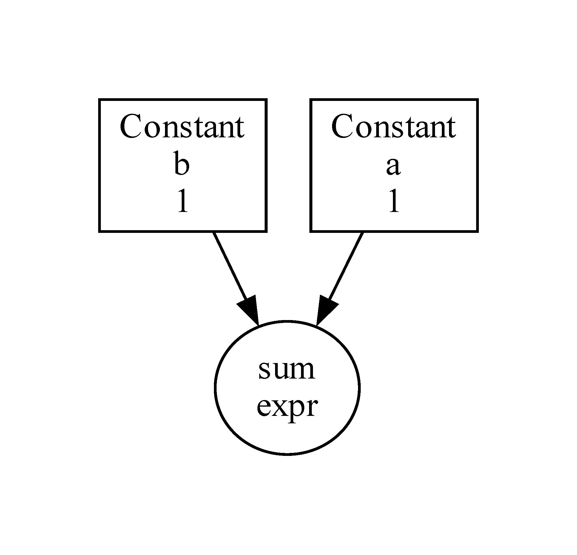
a = flow.Constant(1)
b = flow.Constant(1)
c = a + b                           # c = <Operation ...>, no actual computation is done yet
flow.analyze_expr(c, view=True)     # show the dataflow graph
assert flow.compute_expr(c) == 2    # use compute_expr(node) to execute the graph and do actual computation

OptFlow supports control flow. That is, you can create if and for nodes with context mananger flow.IfCond(condition) and flow.ForLoop(N) in the dataflow graph to implement condition and loop. Different from the native if and for statement in Python, they will not run until the graph is executed.

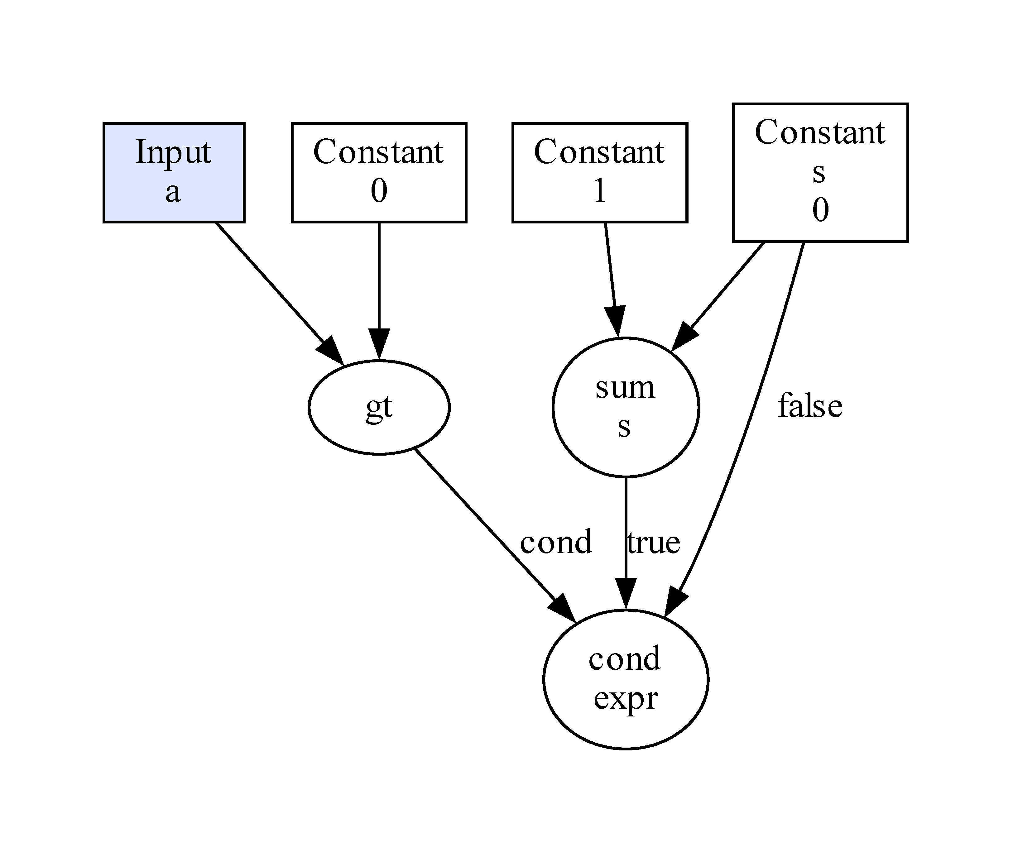
The following example shows how to implement a branch function. The value of s will be added by one if the input node a is larger than 0.

import optflow as flow

s = flow.Constant(0)
a = flow.Input(dtype=flow.int32)    # you can create Input nodes as a placeholder
with flow.IfCond(a > 0):    # no actual "if" condition checking is done yet
    s += 1
res = flow.compute_expr(s, node_value={a: 1})   # feed the value of the Input nodes using a node->value dictionary
assert res == 1
res = flow.compute_expr(s, node_value={a: -1})
assert res == 0

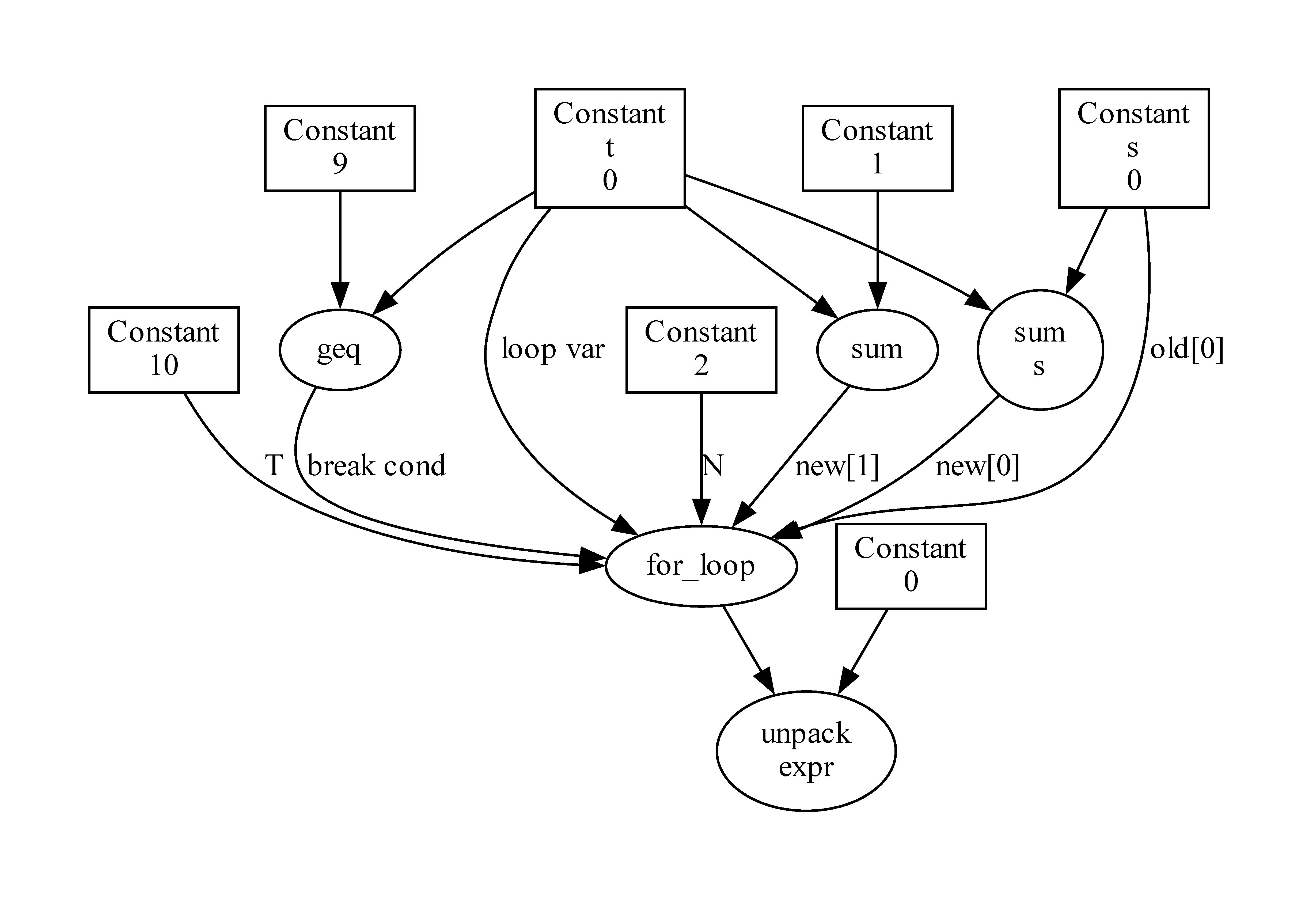
The following code shows how to add number from 0 to 9 with OptFlow dataflow graph.

import optflow as flow

s = flow.Constant(0)
with flow.ForLoop(10) as t:
    s += t
assert flow.compute_expr(s) == 45

Note

The support of control flow makes the dataflow graph Turing-complete. See the example involving a Turing machine for more details.

Describing Optimization Problems using Dataflow Graph#

You can use flow.Problem in OptFlow to create an optimization problem. It has three main components:

objective: a node in the dataflow graph that you want to maximize or minimize.
constraints: a list of boolean nodes in the dataflow graph that need to be satisfied (i.e., values are True) during the optimization.
sense: flow.maximize or flow.minimize, specifying whether you want to maximize or minimize the objective.

Usually, the objective and constraints are functions of some decision variables. You can create decision variables in OptFlow via flow.Variable. It has the following parameters:

cat: the category of the variable, which can be set as
- flow.binary: 0 (false) or 1 (true)
- flow.categorial: 0, 1, …, N (you should also specify N via the size parameter), can be used as index of arrays
- flow.continuous: any non-negative float number
- flow.integer: any non-negative integer, a descrete version of flow.continuous, cannot be used as index of arrays
- flow.permutation: the permutation of some given elements (you should also specify elements as an integer list in the parameter)
shape: a tuple specifying the shape of the variable.
size (only for cat=flow.categorial)
elements (only for cat=flow.permutation)

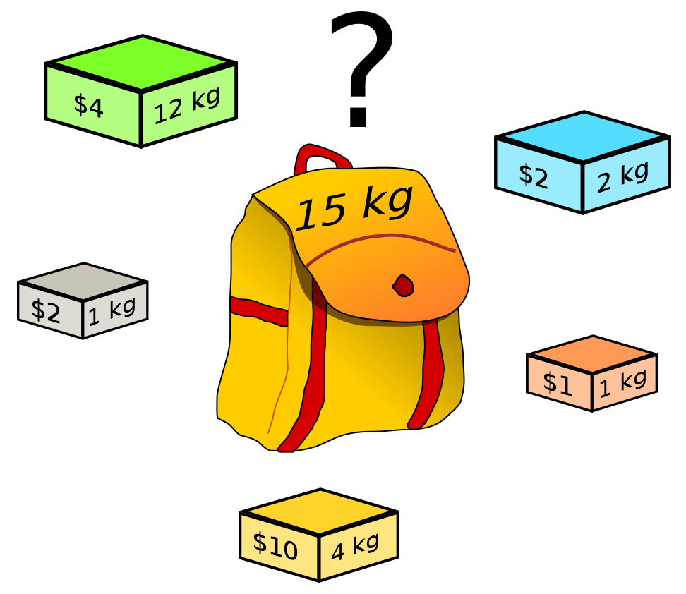
We start from a simple knapsack problem. Consider that we have 5 boxes with specific size and weight

https://commons.wikimedia.org/wiki/File:Knapsack.svg

	box 1	box 2	box 3	box 4	box 5
weight (kg)	12	2	1	4	1
value ($)	4	2	1	10	2

Then, which boxes should be chosen to maximize the amount of money while still keeping the overall weight under or equal to 15 kg?

We can use five binary decision variables to describe this problem in OptFlow as follows:

import numpy as np
import optflow as flow

# x[i] = 1 if the ith items is in the knapsack, x[i] = 0 otherwise
x = flow.Variable(flow.binary, shape=(5,))
weight = flow.Constant(value=np.array([12, 2, 1, 4, 1], dtype=int))
value = flow.Constant(value=np.array([4, 2, 1, 10, 2], dtype=int))

total_weight = flow.sum([weight[i] * x[i] for i in range(5)])
total_value = flow.sum([value[i] * x[i] for i in range(5)])
# we require the total weight not exceeding the size of the knapsack
constraints = [total_weight <= 15]

prob = flow.Problem(
  objective=total_value,
  constraints=constraints,
  sense=flow.maximize
)
prob.visualize()

Solving Optimization Problems with Different Optimization Methodologies#

We can use the solve method of a flow.Problem instance to solve a problem. OptFlow supports multiple optimization methodologies to solve a problem, each has their specific range of application and some of them are AI-assisted. You can specify the paradigm via the solver parameter. Currently, OptFlow have three optimization methodologies available for general optimization problems:

flow.search: OptFlow will traverse through full or part of the solution space via search algorithm, for combinatorial optimization (all variables should be discrete).
flow.programming: OptFlow will apply linear programming / MIP solver, for problem with linear objective and constraints. Note that the control flow in OptFlow is not fully supported in this mode. Please consider using the native Python if and for statement to describe the problem.
flow.metaheuristics: OptFlow will generate an initial solution and apply metaheuristics algorithms to refine the solution iteratively, for combinatorial optimization.

For the knapsack problem mentioned above, we can use the following optimization methodologies to solve it:

prob.solve(solver=flow.search)
print(x.optimized_value)    # [0 1 1 1 1], indicating that we should select box 1, 2, 3, 4, not 0
prob.solve(solver=flow.programming)  # since the objective and constraints are all linear, we can also apply mathematical programming solver
print(x.optimized_value)    # [0 1 1 1 1]
prob.solve(solver=flow.metaheuristics)  # metaheuristics is also available for combinatorial optimization
print(x.optimized_value)    # [0 1 1 1 1]

Describing Sequential Optimization Problems using Dataflow Graph#

Many optimization problems can be naturally described as a sequential process. That is, you make your decision step by step, and you want to optimize your decisions with respect to a specific objective. For example:

For the knapsack problem described above, we can make a 5-step decision. On step i we decide whether to include box i into the knapsack.
For Traveling Salesman Problem on a graph of N cities, we can make an N-step decision. On step i we decide which city to go
For the maze problem in which we want to find a shortest valid route in a grid world toward the exit, we can make stepwise decisions. In each step we decide which direction to go (up, down, left, right)
…

In OptFlow, we describe a sequential optimization problem in a flow.ForLoop context, such as

obj = flow.Constant(0.)
constraints = []
with flow.ForLoop(T) as t:
  constraint.append(...)    # add constraint in the FOR loop
  ...                       # describe the problem logic of each step in the FOR loop
  obj += ...                # update the objective in the FOR loop
  
prob = flow.Problem(
  objective=obj,
  constraints=constraints,
  sense=...
)

For the knapsack problem, we can describe it in a sequential form as follows

import numpy as np
import optflow as flow

x = flow.Variable(flow.binary, shape=(5,))
weight = flow.Constant(value=np.array([12, 2, 1, 4, 1]))
value = flow.Constant(value=np.array([4, 2, 1, 10, 2]))

total_weight = flow.Constant(0)
total_value = flow.Constant(0.)
constraints = []
with flow.ForLoop(5) as t:      # a 5-step decision
  with flow.IfCond(x[t]):       # if we include box i into the knapsack
    constraints.append(total_weight + weight[t] <= 15)  # box i should fit the size of the knapsack    
    total_weight += weight[t]   # update the total weight
    total_value += value[t]

prob = flow.Problem(
  objective=total_value,
  constraints=constraints,
  sense=flow.maximize
)
prob.visualize()    # show the dataflow graph

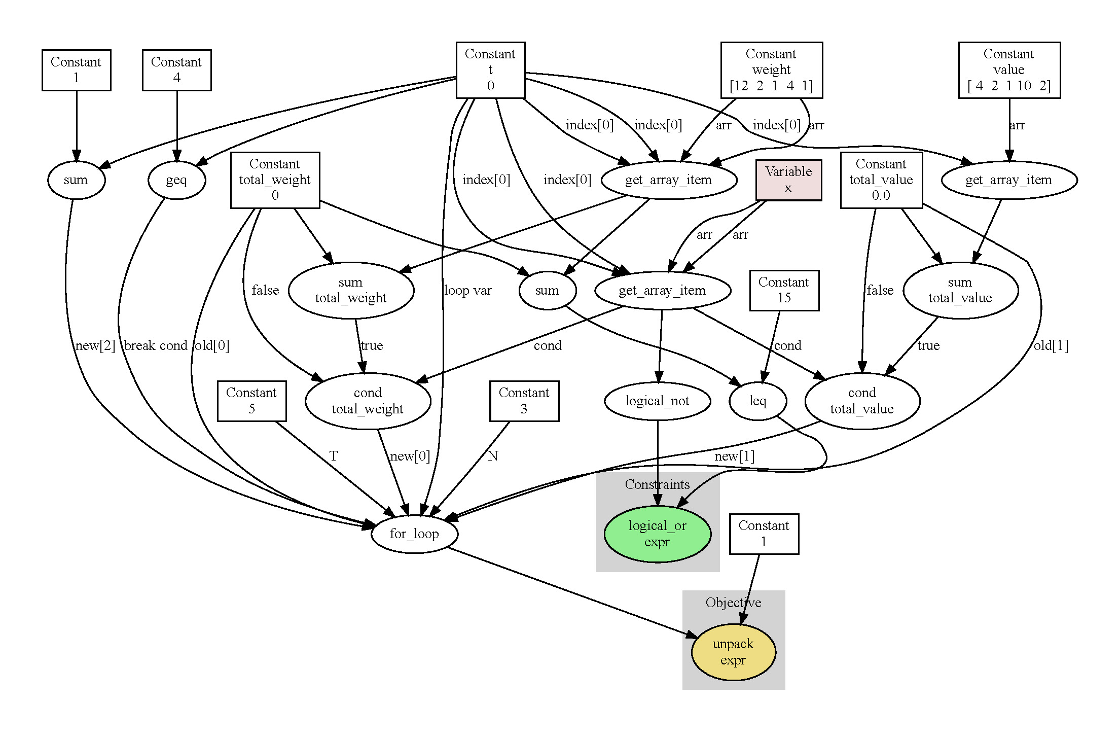
Solving Sequential Optimization Problems with DP and RL#

For optimization problems with such a sequential form, OptFlow has specific optimization methodologies to solve them, including

flow.dp: OptFlow will convert the dataflow graph as a Markov Decision Process and apply dynamic programming to solve it. All the nodes except the objective should be discrete.
flow.rl: OptFlow will convert the dataflow graph as a Markov Decision Process, train a policy on the MDP with reinforcement learning, and use the trained policy to inference the solution.

prob.solve(flow.dp)
print(x.optimized_value)    # [0 1 1 1 1]

prob.train(flow.rl)         # RL requires training before solving
prob.solve(flow.rl)
print(x.optimized_value)    # [0 1 1 1 1]

JIT Compilation to Accelerate Solving#

For optimization methodologies requiring frequent interaction or evaluations with user-defined functions, such as metaheuristics and reinforcement learning, OptFlow is able to accelerate the solving process with Just-in-Time compilation techniques. More specifically, OptFlow implements a Just-in-Time compiler based on LLVM that compiles a specific part or all of the dataflow graph into efficient native machine bytecode, that can be optimally run on users’ current computation device.

To enable Just-in-Time compilation, you can add an 'jit': True key-value pair in the params parameter of Problem.solve() or Problem.train(). For example,

opt_obj = prob.solve(solver=flow.metaheuristics, params={'jit': True})

Note

This is an experimental feature in development. Not all opeartors are supported yet.

An online example of JIT acceleration is available [here] (password: )