Traveling Salesman Problem (TSP)#
The following code shows how OptFlow solves the knapsack problem with mathematical programming and search
# Author: Anonymized for paper review
# Case Study: Traveling Salesman Problem

import optflow as flow
import numpy as np

N = 4
D = flow.Input(dtype=flow.ndarray, shape=(N, N))
x = flow.Variable(cat=flow.categorical, size=N, shape=(N - 1, ))
x_init = flow.Constant(dtype=flow.categorical, size=N, value=0)
loc = flow.Set(size=N)
loc = flow.set_add(loc, x_init)
obj = flow.Constant(value=0.)
constraints = []
for t in range(N - 1):
    constraints.append(flow.set_not_in(loc, x[t]))
    loc = flow.set_add(loc, x[t])
    if t == 0:
        obj = obj + D[x_init, x[t]]
    else:
        obj = obj + D[x[t - 1], x[t]]

# search
flow.solve(constraints=constraints, objective=obj, sense=flow.minimize, solver=flow.search,
           inputs={D: np.array([[0, 2, 1, 1], [2, 0, 1, 1], [1, 1, 0, 2], [1, 1, 2, 0]])})
for i in range(N - 1):
    print(x[i].optimized_value)

# programming
flow.solve(constraints=constraints, objective=obj, sense=flow.minimize, solver=flow.programming,
           inputs={D: np.array([[0, 2, 1, 1], [2, 0, 1, 1], [1, 1, 0, 2], [1, 1, 2, 0]])})
for i in range(N - 1):
    print(x[i].optimized_value)
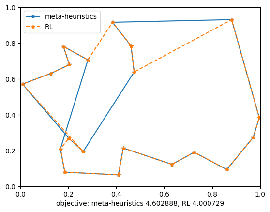
The following code shows how OptFlow solves the problem with metaheuristics and model-free reinforcement learning, which requires the problem to be represented as a sequential one

Note
The RL method introduced in the following VRP paper will be automatically applied to the problem when RL is selected, as OptFlow detected the VRP structure of the problem.
M. Nazari, A. Oroojlooy, L. Snyder, and M. Takac, “Reinforcement Learning for Solving the Vehicle Routing Problem,” in Advances in Neural Information Processing Systems, 2018, vol. 31. [Online]. Available: https://proceedings.neurips.cc/paper/2018/hash/9fb4651c05b2ed70fba5afe0b039a550-Abstract.html
import optflow as flow
import numpy as np
import scipy.spatial
import matplotlib.pyplot as plt

N = 20
city_coords_ = np.random.rand(N, 2)
dist_ = scipy.spatial.distance_matrix(city_coords_, city_coords_)

city_coords = flow.Input(dtype=flow.ndarray, shape=(N, 2))
dist = flow.Input(dtype=flow.ndarray, shape=(N, N))
x = flow.Variable(cat=flow.permutation, size=N, shape=(N, ), elements=list(range(N)))
visited = flow.Constant(dtype=flow.binary, shape=(N, ), value=np.array([False] * N))
obj = flow.Constant(value=0.)
start_pos = flow.Constant(dtype=flow.categorical, size=N, value=0)
last_pos = flow.Constant(dtype=flow.categorical, size=N, value=0)
constraints = []

graph = flow.Graph(num_nodes=N, adjacent_matrix=dist, node_attributes={
    'city_coords': city_coords,
    'visited': visited
})

# input: dist (location, not changed during the sequential process)
# state: start_pos, last_pos, visited, (obj, t)
# task: build an optimal mapping (policy) from state to action (x[t])
# to enhance the generalization performance over different inputs,
# actually we need to build a mapping from (state, input) to action (x[t])
# even if the input will not change during a specific sequential process
with flow.ForLoop(N) as t:
    constraints.append(flow.logical_not(visited[x[t]]))
    with flow.IfCond(t == 0):
        start_pos = x[t]
    visited[x[t]] = True
    with flow.IfCond(t != 0):
        obj += graph.distance(last_pos, x[t])
    last_pos = x[t]
    with flow.IfCond(flow.reduce_sum(visited) == N):
        obj += graph.distance(x[t], start_pos)
        flow.break_loop()

prob = flow.Problem(objective=obj, constraints=constraints, sense=flow.minimize)

class DataGenerator(flow.DataGenerator):
    def __init__(self, N):
        self.N = N

    def __call__(self):
        city_coords_ = np.random.rand(self.N, 2)
        dist_ = scipy.spatial.distance_matrix(city_coords_, city_coords_)
        return {dist: dist_, city_coords: city_coords_}


# prob.train(flow.rl, inputs_generator=DataGenerator(N))
prob.load_model(r'tsp_20_checkpoint')
opt_obj_rl = prob.solve(flow.rl, inputs={dist: dist_, city_coords: city_coords_})
res_rl = list(x.optimized_value)
res_rl.append(res_rl[0])
print(x.optimized_value, opt_obj_rl)

opt_obj_meta = prob.solve(flow.metaheuristics, inputs={dist: dist_, city_coords: city_coords_})
res_meta = list(x.optimized_value)
res_meta.append(res_meta[0])
print(x.optimized_value, opt_obj_meta)

plt.plot(city_coords_[res_meta, 0], city_coords_[res_meta, 1], "*-", label='meta-heuristics')
plt.plot(city_coords_[res_rl, 0], city_coords_[res_rl, 1], "*--", label='MDP')
plt.xlim(0, 1)
plt.ylim(0, 1)
plt.legend()
plt.xlabel("objective: meta-heuristics %f, RL %f" % (opt_obj_meta, opt_obj_rl))
plt.show()
[Run Online Demo] (password:  )
)